When Did That Hotspot Happen?
- The Flamegraph Lie
- What You Actually Want
- stackprofile
- Reading the Output
- Bursty vs Steady: A Concrete Difference
- Flamegraph vs stackprofile
- Prior Art and How stackprofile Differs
- For AI Agents Too
- Where It Shines
- Try It
The Flamegraph Lie
Flamegraphs are the standard answer to “where is the CPU going?” You get a beautiful tree of call stacks, widths proportional to sample counts, and you can visually spot the methods that dominate. It is a deservedly popular visualization.
But a flamegraph aggregates everything. Two minutes of recording become one static picture. A method that burned 10% of CPU for two straight minutes looks exactly the same as a method that burned 100% of CPU for twelve seconds and was idle for the rest. Both show the same width in the graph. Both report the same sample count.
This matters more than you might think. The first case is a steady load, probably a core loop doing its job. The second is a burst, maybe a periodic batch, a cache rebuild, a sudden queue drain. The diagnosis is different, the fix is different, and the urgency is different. But in a flamegraph, they are the same rectangle.
What You Actually Want
When you find a hot method in a profile, the next questions are almost always temporal:
- Was it hot the entire time, or only during a spike?
- Is it one thread doing all the work, or is it spread across many?
- Is this a steady-state cost I should optimize, or a transient burst I should investigate?
None of these questions can be answered by a tool that throws away the time axis.
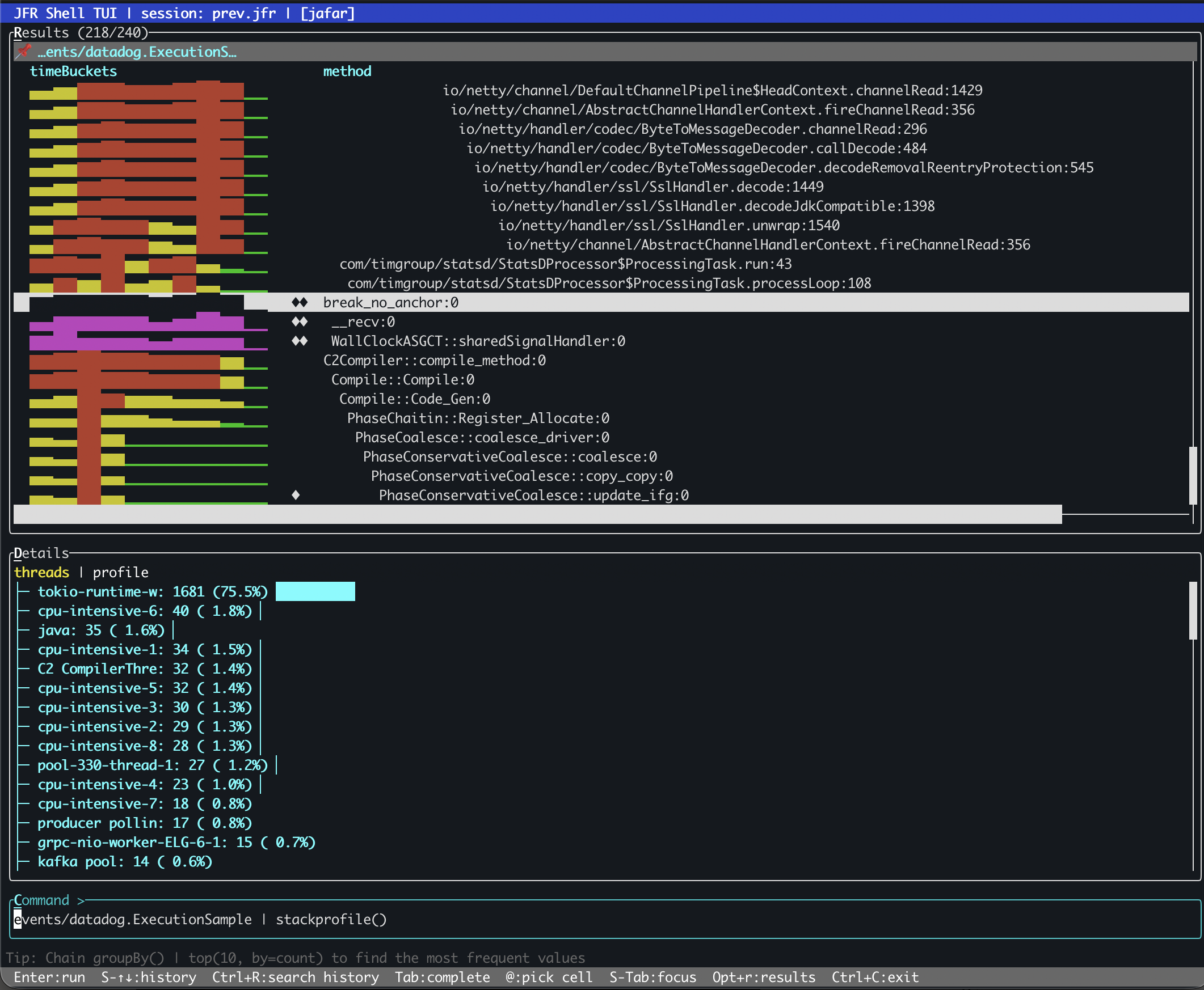
stackprofile
jfr-shell now has a stackprofile pipeline operator that keeps the time axis. Instead of collapsing all samples into a single tree, it builds a weighted call tree where every node carries two extra pieces of information: a time-bucket distribution showing how samples spread over the recording duration, and a per-thread breakdown showing which threads contributed.
The syntax is what you would expect from a pipeline operator:
events/jdk.ExecutionSample | stackprofile()
It accepts a few optional parameters:
| Parameter | Default | Meaning |
|---|---|---|
direction |
top-down |
top-down for caller paths, bottom-up for hot methods first |
buckets |
10 |
Number of time buckets across the recording |
minPct |
1.0 |
Minimum percentage threshold, prunes noise |
A bottom-up view with finer time resolution:
events/jdk.ExecutionSample | stackprofile(direction=bottom-up, buckets=20, minPct=0.5)
Reading the Output
Each row in the result is a frame in the call tree, annotated with:
- total: samples in this frame or any of its children
- self: samples where this frame is the leaf (the actual work)
- time buckets: a sparkline showing sample distribution across the recording
- threads: per-thread sample counts with percentages
The operator also classifies each frame into a category:
| Marker | Category | Meaning |
|---|---|---|
| (none) | normal |
Below 1% self time |
◆ |
hotspot |
1%+ self time, bursty or intermittent |
◆◆ |
steady-hotspot |
1%+ self time, uniform across all time buckets |
That last category is the interesting one. A steady hotspot is a method that consumes significant CPU at a constant rate for the entire recording. It is not reacting to a spike, it is not processing a batch. It is always there, always burning. These are classic N+1 query candidates, polling loops, or inefficient serialization paths. They are the kind of thing that flamegraphs make look “normal” because they blend into the background.
Bursty vs Steady: A Concrete Difference
Consider two methods that each account for 5% of total CPU in a two-minute recording:
Method A — steady hotspot:
time buckets: ▃▃▃▃▃▃▃▃▃▃  (uniform across all 10 buckets)
threads:      worker-1 (40%), worker-2 (35%), worker-3 (25%)
category:     ◆◆ steady-hotspot
This method is always running, spread across multiple worker threads. It is a baseline cost. If you want to reduce CPU, this is a method worth optimizing because the savings compound across the entire recording.
Method B — bursty hotspot:
time buckets: ▁▁▁▁▁▁▁█▁▁  (concentrated in bucket 8)
threads:      batch-processor-1 (100%)
category:     ◆ hotspot
Same percentage, completely different story. This method fired once, in a single burst, on a single thread. It is probably a scheduled task, a cache refresh, a one-time computation. Optimizing it would save nothing during normal operation. The right response might be to move it off the hot path or run it at a less contended time.
A flamegraph cannot tell these apart. stackprofile can, because it kept the time axis.
Flamegraph vs stackprofile
The two operators complement each other. Neither replaces the other.
| Dimension | flamegraph |
stackprofile |
|---|---|---|
| Output | Aggregated call paths | Call tree with temporal metadata |
| Time axis | Collapsed | Preserved (bucketed) |
| Thread info | Not tracked | Per-frame thread breakdown |
| Best for | “Where is CPU going?” | “When and on which threads?” |
| Pattern detection | No | Steady vs bursty vs intermittent |
| Format | Folded stacks or tree (visual) | Structured table or JSON (analytical) |
Use flamegraph when you need to understand call paths and caller-callee relationships. Use stackprofile when you need to understand temporal behavior and thread affinity.
Prior Art and How stackprofile Differs
The idea of adding a time axis to profiling data is not new. Several tools have tried different approaches:
-
Flame Charts (Chrome DevTools, Polar Signals) preserve temporal ordering by not merging stacks at all. Every individual call is shown in time sequence. This is faithful to the recording, but for a two-minute JFR with tens of thousands of samples, the result is too noisy to navigate. You get time, but you lose the ability to spot patterns.
-
Differential Flame Graphs (Brendan Gregg) compare two profiles, A and B, coloring frames red or blue based on the delta. Great for before/after comparisons, but they only answer “did this method get hotter or colder between these two snapshots?” They cannot show a continuous temporal distribution within a single recording.
-
dotTrace Timeline Profiling (JetBrains) gives a full thread-level timeline with call stacks at each point. Powerful, but .NET-only, and it is a GUI tool rather than a composable pipeline operator.
-
binjr can browse JFR method profiling events as time series and show histogram density distributions. It gives you the temporal view, but it works at the individual event level rather than aggregating into a call tree.
stackprofile takes a different path. It merges stacks like a flamegraph (keeping the output compact and navigable) but annotates every node in the tree with a bucketed time distribution and per-thread breakdown. You get the structural clarity of a merged call tree plus the temporal insight of a flame chart, without the noise of either extreme.
For AI Agents Too
stackprofile is also exposed as an MCP tool (jfr_stackprofile) through jfr-mcp. The MCP version returns structured JSON with numeric fields for every frame: totalPct, selfPct, pattern, category, timeBuckets array, and threadCounts map. This makes it straightforward for an AI agent to programmatically identify bursty hotspots, detect N+1 patterns, or compare thread affinity across frames without parsing sparklines.
claude mcp add jafar -- jbang jfr-mcp@btraceio --stdio
Then ask Claude to investigate temporal CPU patterns, and it will use jfr_stackprofile alongside jfr_flamegraph and jfr_hotmethods to build a more complete picture.
Where It Shines
stackprofile works in the plain CLI, but its full potential shows in two places: the TUI and MCP.
In TUI mode, the results are color-coded by category. Normal frames stay neutral, hotspots get highlighted, and steady-hotspots are immediately visible. You can jump directly to the next hotspot without scrolling through hundreds of normal frames. When a recording has thousands of frames, that navigation alone saves real time.
Through MCP, an AI agent gets structured JSON with numeric fields it can reason over programmatically. It can scan for steady-hotspots, compare thread affinity across frames, and detect N+1 patterns without parsing visual output. The combination of jfr_stackprofile with jfr_flamegraph and jfr_hotmethods gives the agent three complementary views of the same CPU data.
The plain CLI gives you the data. The TUI makes it navigable. MCP makes it queryable by machines.
Try It
# Install via JBang, open a recording
jbang jfr-shell@btraceio -f recording.jfr --tui

# Top-down call tree with temporal bucketing
jfr> events/jdk.ExecutionSample | stackprofile()

# Bottom-up hot methods with 20 time buckets
jfr> events/jdk.ExecutionSample | stackprofile(direction=bottom-up, buckets=20)

# Only frames above 2% of total
jfr> events/jdk.ExecutionSample | stackprofile(minPct=2.0)
The next time you find a hot method in a flamegraph, ask yourself: was it hot the entire time, or just for a moment? stackprofile will tell you.
jfr-shell is part of JAFAR and available via JBang and Maven Central.